Getting started¶

Install¶

Requires Python 3.9 or later. Check your version with python3 --version, then install pyRUMP from PyPI:

pip install pyrump

numpy, scipy, and matplotlib are installed automatically, along with the physics data tables pyRUMP needs at runtime.

Quick start¶

pyrump                         # the interactive shell, from any directory

Data loading¶

Anything ending in .rbs/.RBS might be one of two unrelated things: RUMP's own binary spectrum format, or a plain-text acquisition macro that just happens to share the extension. GET and XEQ load them, respectively — using the wrong one gets you a clear error rather than garbage data. See File formats in the manual for the full specification of both.

Example 1 — RUMP binary format (.rbs)

examples/2A.rbs is a real binary spectrum (Cornell format, mode-2 differential-compressed counts):

Your wish? cd examples
Your wish? get 2A.rbs
active buffer is now 1

GET decodes the file's records directly — calibration, geometry, accelerator settings and the 2048 channel counts all arrive in one call. The spectrum lands in buffer 1: in RUMP, buffer 1 is always "whatever was read most recently," not a fixed slot, and every other data buffer shifts up one to make room (buffer 0 is reserved for the simulation and is never touched by GET). Buffer 1 also becomes the active buffer, so PLOT, COMPARE, INTEGRAL and friends act on it right away:

Your wish? active
Buffer 1:
  File       2A.rbs
  Identifier Binghampton_target_02A.RBS  RBS LT =  905.98 RT  962.42
  ...
Your wish? plot 1

Example 2 — an acquisition macro under a .RBS extension

Some acquisition software (NEC's RC43 among them) writes its output as a plain-text EMPTY/SWALLOW command macro named something.RBS, despite the name suggesting real spectrum data. examples/MnPt.RBS is one of these — load it with XEQ, not GET:

Your wish? xeq MnPt.rbs
buffer 1 emptied
  c:\RBS\data\2022\01\MnPt.RBS
  MnPt.RBS  170 Degree RBS LT =  2457.874 RT  2463.078 Gain  2
  ...
2048 points entered into buffer 1

XEQ replays the file line by line through the same command interpreter as the prompt: it sets IDENTIFIER, DATE, CONVERSION, the beam and geometry, then hits SWALLOW, which reads every following line as channel data straight into the buffer — landing in buffer 1 exactly like GET does.

Loading either file with the wrong command fails loudly instead of silently misreading it:

Your wish? get MnPt.rbs
could not read .../MnPt.RBS: .../MnPt.RBS is a text command macro
(RC43's EMPTY/SWALLOW convention), not a binary RUMP spectrum -- use XEQ,
not GET, to load it

Your wish? xeq 2A.rbs
.../2A.rbs is not a text command file (...) -- binary spectrum data belongs
with GET, not XEQ

Plotting¶

Picking up with buffer 1 already loaded (either example above works), PLOT opens one persistent matplotlib window whose state survives between commands:

Your wish? plot 1               /* erase and plot buffer 1             */
Your wish? region 100 400       /* zoom to a channel range             */
Your wish? sqrt                 /* sqrt yield scale, redraws right away */

See Plotting & display in the manual for the rest — OVERLAY, COMPARE, EXPAND, LOG/LINEAR/SQRT, ENERGY, FIGSAVE and more.

Simulating with SIM¶

SIM edits the sample description that COMPARE and PERT fit against. examples/MnPt.lcm is a real 5-layer description for the spectrum loaded above — SIM GET/SIM SHOW work as one-shots, with no need to enter the SIM sub-level for a quick look:

Your wish? sim get MnPt.lcm
read MnPt.lcm: 5 layers
Your wish? sim show
 >  1            40 A        Ru 1
    2           331 A        Mn 2.73 Pt 1
    3            40 A        Ru 1
    4           330 A        Si 1 O 2
    5          1000 nm       Si 1
  maxpth 1000   straggle 0   multiple 0   absorber 0
Your wish? compare              /* data vs. simulation, with residuals */

Buffer 0 is always the simulation and recomputes itself whenever the sample or the active buffer's parameters change — there is no "simulate" command, exactly as in the original.

See SIM and PERT in the manual for the full SIM command set — editing layers interactively, depth-profile equations, straggling and more.

Fitting with PERT¶

PERT picks which sample and instrument parameters may vary and over which channel window, then fits them by least squares. examples/MnPt.pert is a saved selection for the sample above; GET ... GO replays it and runs the fit in one line:

Your wish? pert get MnPt.pert go
  ...
  Fitting MnPt: Si [1000nm] - SiO2 [330A] - Ru [40A] - Mn2.73Pt [331A] - Ru [40A]

  fit took 0.18 s

  reduced chi-square 12.3538 on 397 dof
  35 evaluations, `xtol` termination condition is satisfied.
  kev(0)                            48.4324  +/- 0.04736   (was 48)
  layer 2 thickness                     250  +/- 0.5042   (was 254)
  layer 2 composition Mn             2.8231  +/- 0.01217   (was 2.73495)
  fwhm                              24.9921  +/- 0.03427   (was 15)

  MnPt: Si [1000nm] - SiO2 [330A] - Ru [40A] - Mn2.82Pt [326A] - Ru [40A]

Fitted values are written back into the sample description (SIM SHOW reflects them), and COMPARE shows how the result actually matches the data:

Your wish? region 300 1130      /* zoom to the fitted window            */
Your wish? compare              /* data vs. simulation, with residuals  */
Your wish? figsave fit.png

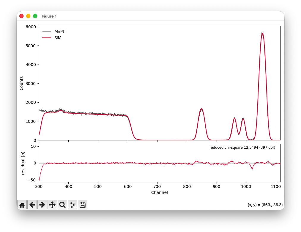
MnPt data vs. the fitted simulation, with residuals

See SIM and PERT in the manual for the full PERT command set — bounded fits, WINDOW/NORMALIZE, REPORT, and the composition-degeneracy caveat worth reading before your first real fit.

Command line¶

You can drive pyRUMP as one-off batch commands, without the interactive shell:

pyrump simulate sample.lcm --energy 2.0 --beam 4He -o out.rbs
pyrump fit sample.lcm measured.rbs --vary thickness:0 --window 190 226
pyrump plot measured.rbs --compare out.rbs -o comparison.png
pyrump convert measured.rbs measured.dat

See CLI reference for every option, or Python API to call the library directly.